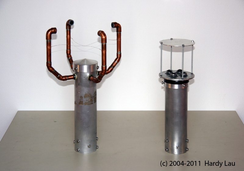
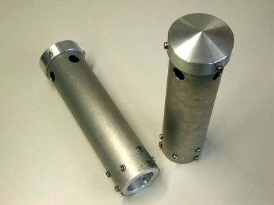
Picture: Both prototypes side by side.
This side describes my own development of a precision measuring ultrasonic wind sensor. This prototype instrument is operating equal good as several commercial devices. Please read in addition also my conclusion at the end of this page.
Picture: Both prototypes side by side.
All rights reserved!
Two different prototypes have originated. At advancement, you can see the innovations with the second version.
This page is no construction manual, but the short description of the development created over a time of 10 years. The mathematical methods can be only mentioned in this shortness and assume to the understanding generally an appropriate university study. However, nobody should hold this from reading this small article. But I cannot deepen the mathematical bases further. However, besides, I have tried to provide references (often Wikipedia) for an explanation.
It concerns here a developing draft. I am glad about corrections or suggestions. Maybe somebody also likes to improve my translation into the English language.
Since 2010, I worked on the advancement.
The work on the second prototype is finished now.
This page is extended over and over again at the most different places.
With interest, a look about the whole page is recommendable now and then.
The last supplement to website: 24st of October 2023
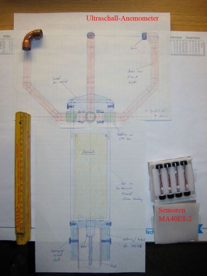 Picture: Sketch of the planned construction (End of 2004). |
 Picture: Result (Mid of 2008). |
| Wind speed | Measuring area | 0..45 m/s | OK |
| Exactness |
±0.3 m/s rms or ±2% rms The bigger value is valid | OK* ** | |
| Resolution | 0.05 m/s | OK | |
| Wind direction | Measuring area | 0... 359° | OK |
| Exactness | ± 2.0° rms (> 5m/s) | OK* | |
| Resolution | 1° | OK | |
| Virtually temperature | Measuring area | -30 °C ... +60 °C (-22 °F ... +140 °F) | OK*** |
| Exactness | ± 1 K (wind < 10 m/s) | OK* | |
| Resolution | 0.1 K | OK | |
| Data output | Interface | RS485 (RS232) | |
| Speed | 19200 baud / 115200 baud (debug) | ||
| Issue | Wind speed, wind direction, (virtual temperature, status) | ||
| Issue rate | 4 per second (WMO) / 1 per second with prototype II | ||
| In general | Internal measuring rate | 400 measurements per second / 80 measurements per second | |
| Power supply | Electronics 13...18 V DC, heating 13...18 V DC, max. 7A | ||
| Protective kind | IP 54 | ||
| Ice formation | With heating mostly prevented | ||
| Mounting | on mast's pipe 50 mms | ||
*) no calibration according to DKD (like NIST).
**) with all calibration factors applied (only prototype II).
***) No explicit output of value with the prototype II up to now.
This ultrasonic anemometer serves for the 2-dimensional capture of the horizontal components of the wind speed and the wind direction as well as the virtual temperature. On account of the high measuring rate, this device is suited very well to capture gusts and peak value measurement without sluggishness. The accessible exactness with the measurement of the air temperature (virtual temperature) partially excels those of the classical procedures with which temperature measuring feelers are used in a weather and radiation protection. The measuring values are provided as data telegrams above a serial interface. All sensors and the device body are heated in freezing. Therefore, the function is also guaranteed with snowfall and ice rain, as well as the possibility of an ice formation is prevented to a great extent.
This ultrasonic anemometer consist of four ultrasonic converters forming two measuring directions orthogonal to each other. The distance is approx. 21 cm. The converters function as a sonic transmitter as well as a sonic receiver. With the start of a measurement a sequence of four single measurements start in all four directions of the measuring distances. The measuring directions (sound propagation directions) proceed rotary. From four single measurements into each direction one wind vector is formed and used to the further calculation. The required time for a measuring sequence is 10 milliseconds.
Even if on this side the time measurement of a short sound impulse appears over and over again, actually, it is a phase measurement with post-regular assignment of the absolute phase by time measurement. The phase is won by a measurement of several zero passageways of the receipt signal in the area of large amplitude after the arrival of the signal. Rushing and a possible offset of the comparator are compensated by the averaging of positive and negative zero passageways.
The correct zero passageway of the phase measurement is assigned by an adaptive digital filter which compares the received signal to a reference signal. A part of the wrapping curve of the signal is evaluated therefore indirectly.
With the time measurement, the essential problem is the recognition of the slow rising amplitude. However, this amplitude and their increase are caused by turbulence in the air which takes away energy, not from the signal consistently. This turbulence is caused among other things by the sound converters itself and is more distinctive with higher wind speed.
If now an amplitude decrease precipitates unexpectedly the threat consist of finding out a jump in the measurements. The error could be to detect the right amplitude a cycle sooner or later within the signal. This leads to wrong wind speeds and temperature measurements.
The solution for this problem is a Kalman-filter. With a digital post-treatment, we incorporated the safety at the detection. Several measurements are required for a two-dimensional capture of wind speed. Besides, e.g., the measured temperature may not be different between both linearly independent directions. The speeds in execution and reverse direction must correspond. Also, the wind speed and temperature can change with a high measuring frequency only limited fast. With all this checks certain detection can be guaranteed.
By the Kalman-filter, the problem exists to begin the evaluation with the right start values at the start or after interruption of the measurement.
And exactly here are the borders. There is a solution only by the advanced possibilities with a larger bandwidth. Read in addition at the advancement.
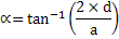
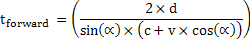
The propagation speed of the sound in calm air overlaps the speed component of an air movement in wind direction. A wind speeds component in the propagation direction of the sound supports its propagation speed, leads to an increase the same, a wind speeds component against the propagation direction leads against it to a reduction of the propagation speed.
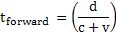

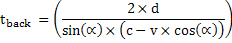
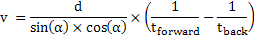
with distance d between the converters, the speed of sound c and wind speed v,
run time of the sound forward tforward and run time of the sound back tback.
From the addition resulting propagation speed leads to different terms of the sound with different wind speeds and directions about a stationary measuring distance. The term of the sound on each of both measuring distances is measured in both directions because the speed of sound is strongly dependent on the temperature of the air. The influence of temperature on the measuring result can be switched off by subtraction of the reciprocal term.
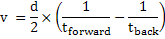
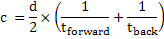
with distance d between the converters, the speed of sound c and wind speed v,
run time of the sound forward tforward and run time of the sound back tback
This representation is valid with the speed of sound (temperature), however, only with calm! (See next below)
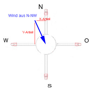
Picture: Arrangement of the sound converters and directions
Afterwards, measurement of the right-angled speed components these are transformed by the microprocessor of the anemometer in polar coordinates and are given as speed and course of the wind.
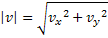
with the amount of the wind speed |v| and two partial wind speeds vx
and vy in the north south or west east directions.
The direction of the wind is won by the use of the trigonometric function arc-tan. Besides, the right quadrant is especially to be considered with the calculation.
The propagation speed of the sound is dependent about a root function on the absolute temperature of the air, however, roughly independent of atmospheric pressure and only slightly depending on the aerial dampness. Hence, this physical connection can be used for a temperature measurement of the air with known and more consistently chemical composition. It concerns, on this occasion, a measurement of the gas temperature without detour of the thermal coupling of this gas to a measuring feeler.
c = 331.5 m/s * √(1 + T / 273.15) with speed of sound c [m/s] and temperature T [°C]
Because of the weak dependence of the propagation speed of the sound of the aerial dampness temperature refers virtually to dry air (0% of dampness) under the same pressure terms.
Tv = c2 / 402.31466 - 273.15 with speed of sound c [m/s] and acoustic virtual temperature Tv [°C]
The divergence measured virtual temperature to the real air temperature is dependent linearly on the absolute moist salary of the air. The portion of the steam in the air leads according to interest to an increase of the speed of sound because H2O molecules own possibly only half of the mass of the remaining aerial molecules (O2 and N2). The increase of the speed of sound leads to a virtual increase of the measured temperature of humid air in comparison to the dry air of the same temperature.
The divergence of the measured virtual temperature of humid air to the real air temperature can be corrected with knowledge of the absolute dampness possibly with the following equation:
Tr = Tv - 0.135 K * m3 / g * a
And Tr shows the real air temperature, Tv the measured acoustic virtual temperature and a the absolute dampness in gram H2O per m3 air. With an air temperature of 20 °C the acoustic virtual temperature with 100% relative dampness is about 2 K too high.
To be able to exhaust all possibilities, an efficient circuit was chosen to exactly capture amplitudes as well as zero passageways and to provide enough compute power.
As a microprocessor, a Microchip dsPIC 30F4012 is used. With 30 MIPS, a 10-bit A/D converters with up to a million samples per second and, in addition, of an analogous zero passageway recognition a measurement and use of the hybrid method is practicable. The times of the zero passageways is captured with the special capture-input. The capture-input and the A/D converter have built-in FIFO memory, so that not every captured value do release an interrupt. The efficiency is so high that even more than 200,000 interrupts per second are no problem. It is possible with this processor to store the amplitude values 500,000 times per second, as well as to capture the times of all zero passageways with a resolution of 34 nanoseconds and to store them. With every single term measurement, all amplitude values of the sound receiver and all times of the zero passageways of the signal are stored and processed only afterwards. The digital signal processor is suitable for the calculation of the correlation very well.
In 2004, this DSP microprocessor was a real innovation. Only the memory size is very limited (2 KB) with this microprocessor (in dip case). The memory size was and, unfortunately, is bound often to the cabinet form.
With the construction of the mechanics and design of the electronics some important points are to be considered.
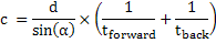
The construction of the analogous circuit requires great care around the rushing slightly to hold. Operation amplifiers from Linear Technology are used. Likewise, a very quick and exact comparator is used by Linear Technology. A DC/DC converter generates the negative voltage and several fixed voltage regulators generate the different supply voltages.
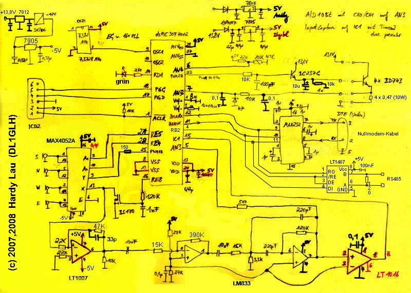
Picture: Complete circuit plan of the first device.

Picture: Screen snapshot of the development system
Now Microchip MPLAB 8.92 and MPLAB C Compiler for PIC24 MCUs and dsPIC v3.31 are used.
It was very hard work to develop this program (2500 lines of c-code). In the present state, it cannot be used directly with
other mechanics.
The parameters and the mismatched filter have to be adapted directly in the code. So the binary is useless for replicas and I will not publish the source code.
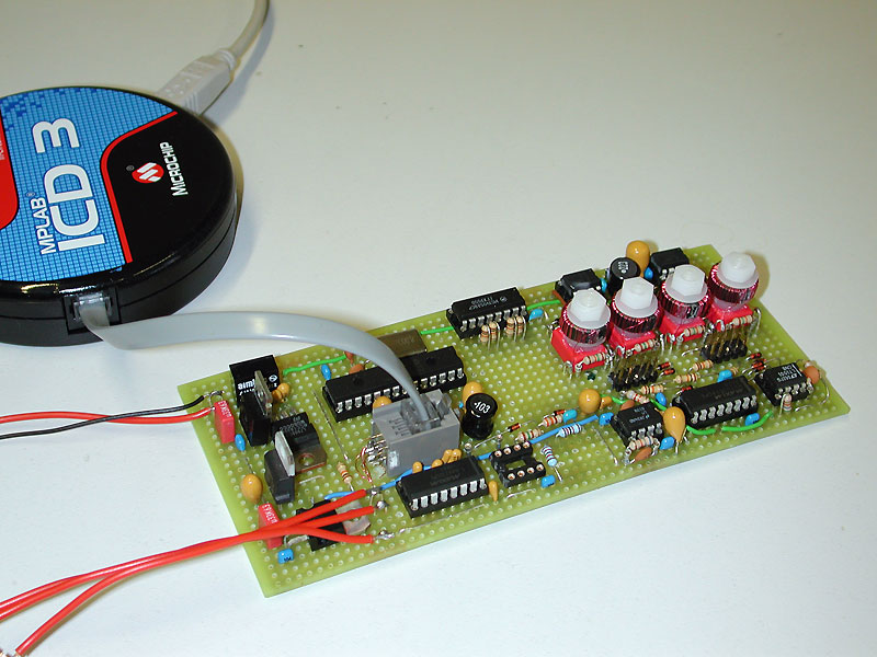
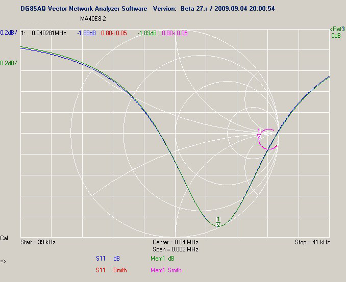
To receive the maximum sound level and to minimize the bell time an adaptation of the transmitters to the sound converters must occur. The sound converter (MA40E8-2) was, therefore, measured with a vector network analyzer.
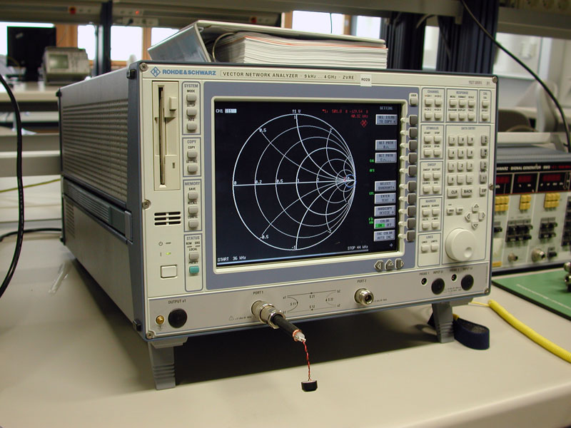
Picture: Rohde & Schwarz network analyzer ZVRE with the measurement of MA40E8-2
 |
 |
 |
| Picture: S11 complex | Picture: S11 real | Picture: S11 phase |
As one can see clearly the frequency of the best adaptation 40.3 kHz is with ambient temperature. Besides, the opposition amounts to approx. 500 ohms. However, the resonance frequency changes conversely to temperature. In the first version, the sound converter is driven directly with 5 Vpp at an impedance of approx. 220 ohms. This is not optimum yet and has caused a lot of problems and wasted a lot of time at the development. Please see also "Advancement" at the bottom of this page.
 Picture: Case without arms. |
 Picture: The lid and the hole for the four arms. |
 Picture: The mast's fixture for a 50 mm pole. The cable entry (not visible) is within the mast's fixture. |
 Picture: Detail of the connection and heating. The white tubes consist of fiberglass. |
 Picture: The glue connections in detail. 3M Scotch-Weld 2216 B/A is used. |
 Picture: The heating transistors |
 Picture: NTC |
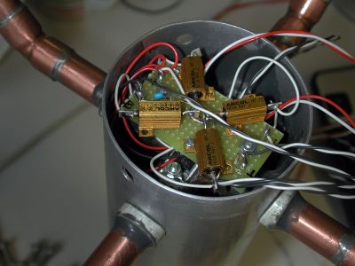 Picture: Shunt resistors assembly for the heating |
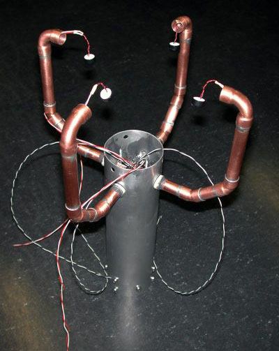 Picture: Shortly before completion of the mechanical construction. |
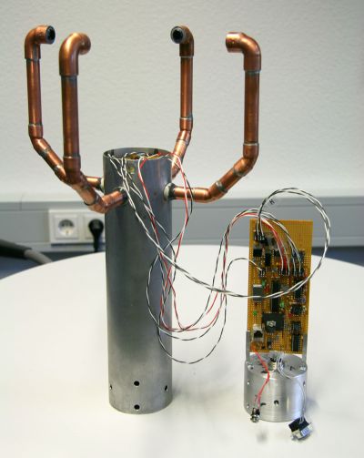 Picture: The device shortly before the assembly. |
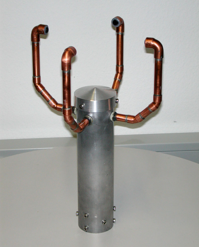
Picture: Ready device
The ultrasound converters are glued with ultraviolet resistant silicone (WEICON Flex+bond).
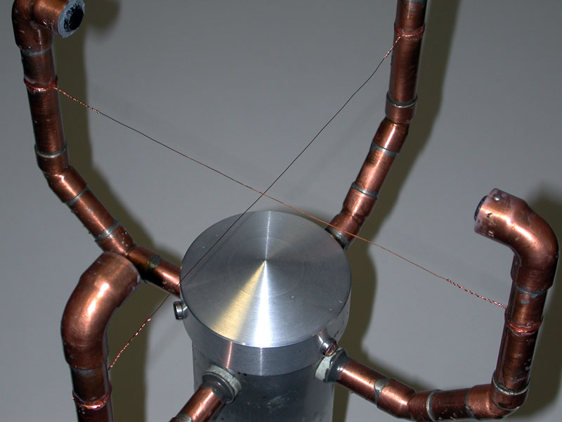
Picture: Protection of birds
The device to refuse large birds was designed to protect the ultrasonic converter from destruction by birds. This device prevents the large birds from sitting on, thus avoiding their interest in the ultrasonic converters. It consists of two metal wires fastened at the ultrasonic sensor arms. Due to the instability of the wires, large birds do not find a safe hold at the instrument.
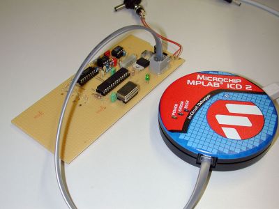 Picture: The DSP processor and the analogous circuit. |
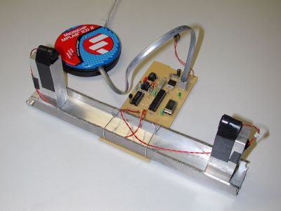 Picture: The first measurements with two sensors. |
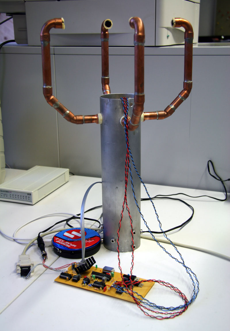
Picture: The converters are pocketed temporarily.
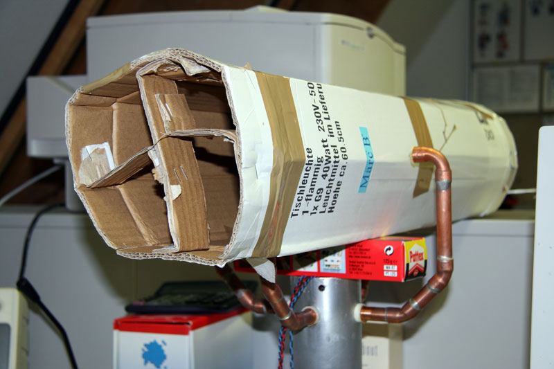
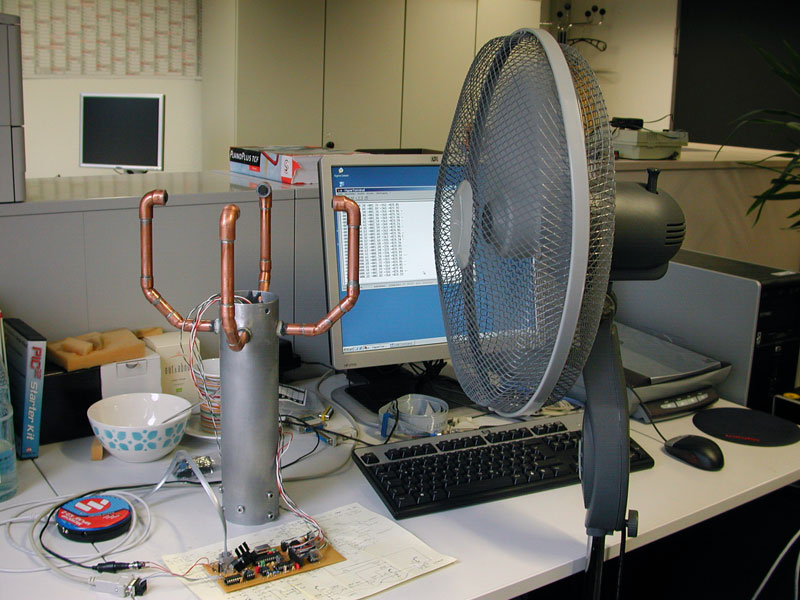
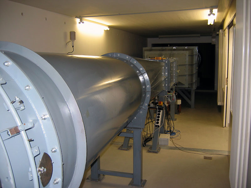
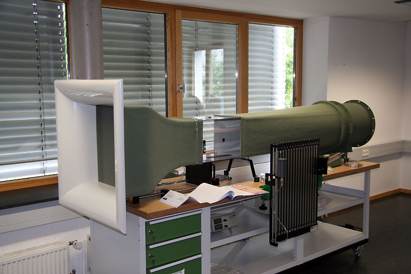
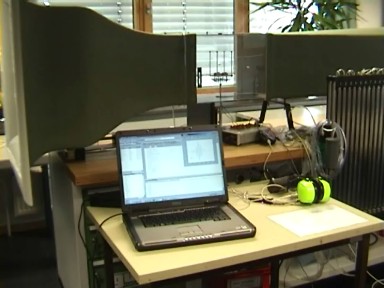
Picture: Primitive wind tunnel
Side view of the wind tunnel for the first test in the lab.
The air is sucked by the channel, thus, there is less turbulence.
The ventilating fan has a supply with up to 28 V with 1.7 A. He is declared with an aerial achievement of 300 cfm. With a canal diameter of 15 cm, a wind speed of 7 m/s (260 cfm) is produced. This speed is also measurable perfectly.
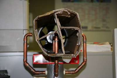 Picture: Front view of the wind tunnel. |
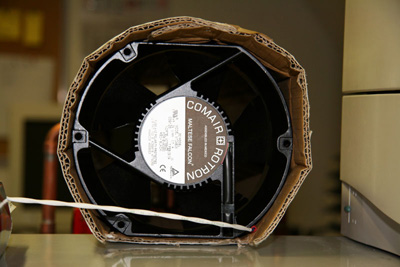 Picture: Back view of the wind tunnel. |
A hybrid attempt is chosen. All times of zero passageways are measured with input capture. The means from several rising and falling zero passageways, at times of the largest amplitude, are calculated. With this averaging the rushing and offset thereby decreases. The precise temporal positions (±n*λ) of the zero passageways are determined by an adaptive digital filter. Besides, the sensor signal is digitized and compared to a stored authoritative signal, using the method of the least squares.
By a pure analogous analysis, the resolution would amount to 2 microseconds, i.e. with 500,000 samples per second approx. 12 samples per wavelength are affected. This is too low, however, is sufficient for a temporal allocation of the zero passageways. By the combination of both procedures, the time resolution amounts to 34 nanoseconds.
Differently expressed the resolution of the wind speed with ambient temperature (20 °C) amounts to 0.02 m/s.
The filtering and processing of the signals are really complex. Following mathematical methods are used:
Picture: The first signal recording with oscilloscope
Picture: Measuring results with the A/D converter (28 measurements in Forward and reverse direction with calm).
Picture: Measuring results with the A/D converter (40 measurements in all 4 directions at approx. 18 m/s in north/south direction).
Picture: Measuring results with the A/D converter (40 measurements in all 4 directions at approx. 27 m/s in north/south direction).
Now you can see that a simple detection based on amplitudes is useless.
Picture: Analysis of the frequency in the signal. After the arrival of the sound pulse, the noise has disappeared. Unfortunately, this cannot be used directly.
Picture: Recording the amplitudes, zero passageways, and mismatched filter
Mathematical analysis of the mismatched filter and calculation of the time from several zero passageways.
Average from several zero passageways is formed at places with big amplitude. The adaptive filter determines
the correct zero passageway. A defined time span earlier (N*λ) the pulse has arrived.
Picture: The least squares proves a clear minimum.
|
Vector h with Nh filter coefficients input u output y We search k for the minimum of y(k) |
Therefore, the method of the least squares was used because the highly optimized library functions (e.g., correlation) of the DSP library work only with 16 bits of values. However, the main memory has not been sufficient for it.
Matched filters obtain best SNR performance in a white Gaussian noise environment but often at the expense of large temporal sidelobes. In radar and ultrasonic applications, large temporal sidelobes can be interpreted as false targets. I use a mismatched filter to minimize temporal sidelobe levels.
And there are the limits of this system. An absolutely perfect detection with all conditions is simply impossible with this low bandwidth. A solution is a larger bandwidth and pulse compression. Read in addition at the advancement.
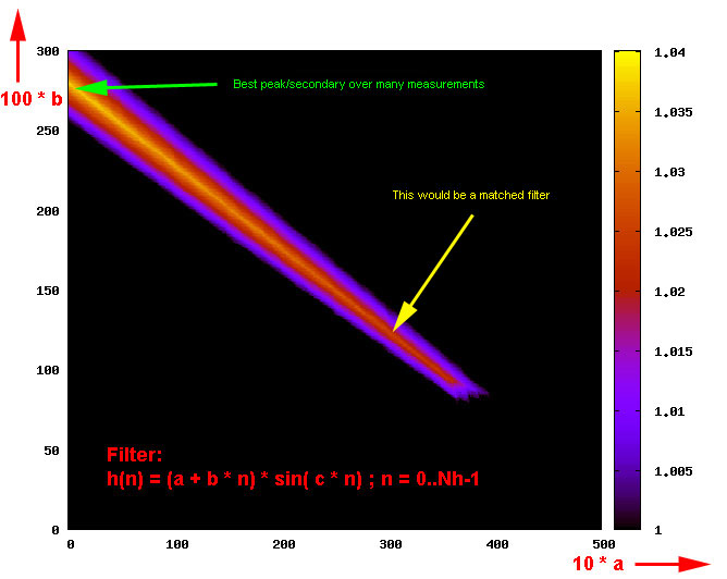
Picture: Optimization of the mismatched filter to the best signal to side lobe.
More about mismatched filters you can read in: "Albrecht Ludloff: Praxiswissen Radar und Radarsignalverarbeitung".
Picture: Variable coefficients of the adaptive filter.
Picture: Vector of wind v, Vector of sound c
The easy representation under "wind speed and direction" is valid strictly speaking only with calm. As soon as the wind vector has accepted an appreciable amount compared with the speed of sound the temperature measurement gets influenced. The sound has to put back a longer way while in each case orthogonal blowing wind deflects the sound. This leads to an enlargement of the term and with it to an ostensible reduction of the temperature. This influencing is dependent on wind direction and wind speed and has to be corrected by the following calculation:
Cx_real = Cx_measured / cos( arctan(|Vy| / Cx_measured) )
with
Cx = Speed of sound in X-direction, |Vy| = Absolute value of wind speed in Y-direction
Cy_real = Cy_measured / cos( arctan(|Vx| / Cy_measured) )
with
Cy = Speed of sound in Y-direction, |Vx| = Absolute value of wind speed in X-direction
Or directly expressed with temperatures:
Tv_x_real = ( Cx_measured2 + Vy2 ) / 402,31466 - 273,15
with
Cx = Speed of sound in X-direction [m/s], Vy = Wind speed in Y-direction [m/s] and T = acoustic virtual temperature [°C]
Tv_y_real = ( Cy_measured2 + Vx2 ) / 402,31466 - 273,15
with
Cy = Speed of sound in Y-direction [m/s], Vx = Wind speed in X-direction [m/s] and T = acoustic virtual temperature [°C]
After the correction, the measured speed of sound (and with it temperatures) should be identical in X direction and Y direction!
Attention: This must be considered by the Kalman-filter!
Picture: Amount of the wind speed with calm
Measurement of the wind speed (in one direction) with calm [in m/s] without averaging.
These are approx. 5000 cycles 4 measurements see. This corresponds with the debug code about 50 seconds.
With suitable averaging the precision still rises because of less rushing.
Picture: Temperature
Measurement of the temperature [in °C] at the same time likewise without averaging.
With suitable averaging the precision still rises because of less rushing.
Picture: Experiment set-up with a ventilating fan as the cheapest wind tunnel.
With this attempt, the ultrasonic anemometer was turned once around the own axis within approx. 48 seconds. The ventilating fan serves as a wind source which generates a very tumultuous wind field.
One can nicely recognize that within 2400 complete measurements (=19200 single measurements) not a single one mistake has appeared.
Picture: Measured temperature course
Picture: Measured speed
Picture: Measured wind direction
Picture: Test of the heating
At the Test of the heating, a step in temperature of more than -50 Kelvin was applied.
The PT1 behavior with a very large dead time can be seen. The regulation behavior is not optimum.
But with wind and precipitation, this is not so important. The temperature at the transducers
is finally +3 °C.
There are two sensible procedures to the average:
This ultrasonic anemometer forms the average of every 1/4 second. Vector average is used at the wind direction and the scalar average is used with wind speed. The differences to the each other procedure are actually unimportant because of the very short time.
After the end of the development, a calibration stands with a measuring instrument always. A difficult task here.
However, an essential part can be carried out without a wind tunnel. The measurement of speed can be tested mostly by measurement of temperature.
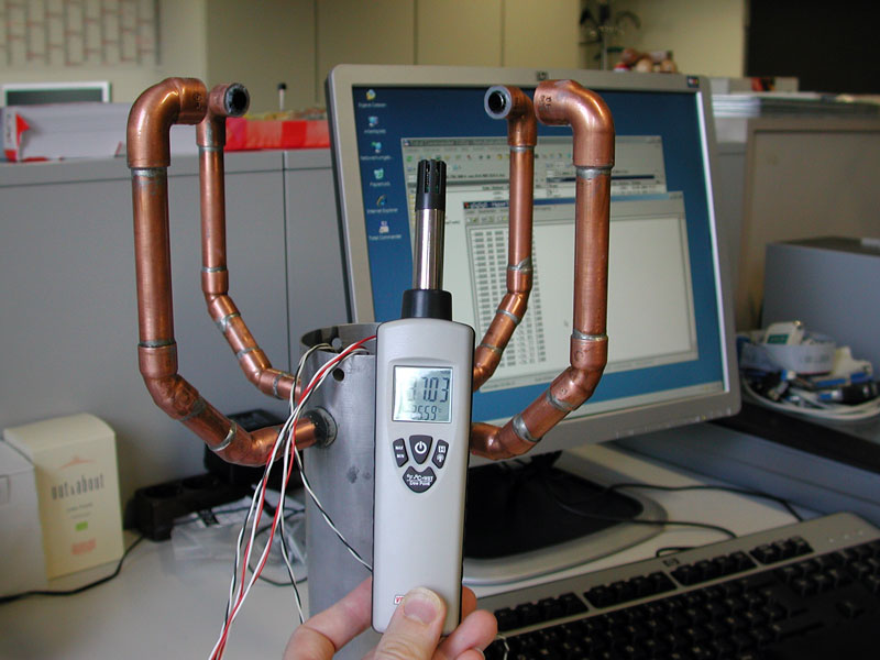
Picture: Measurement of the temperature
Comparative measurement of the temperature. Here an aerial dampness and temperature measuring instrument.
With lab terms (without the wind) tune the measurements of the virtual temperature better than ± 0.5 K.
To remember: If the measured temperature deviates about 6 Kelvin the measuring mistakes with the wind speed amounts to 1%.
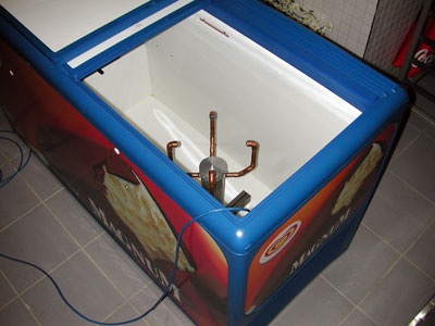
|
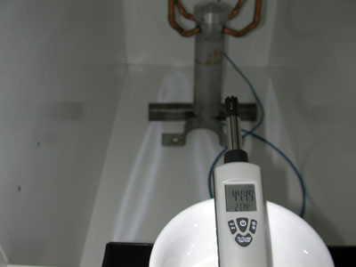
|
Pictures: Temperature tests in a deep fridge down to -30 °C (-22 °F)
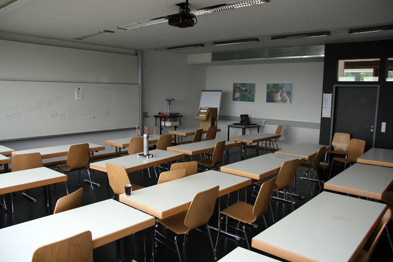
Picture: Measurement in the room
This lecture room was used for the calm and temperature measurements.
However, a thermal balance was not given yet completely, so that a low air movement was possible due to convection.
Picture: Measurement of temperature (60 seconds = 240 values) with averaging (1/4 second) in a closed room.
Picture: Wind vector (60 seconds = 240 values) at the same time in a closed room at nearly calm.
The noise is smaller than 0.01 m/s rms.
The rushing is so slightly, so there is no difference between vector and scalar average.
My car with the shown construction is suited very well as a wind tunnel. The air flow seems totally uninfluenced and laminar.
The problem is the calm.
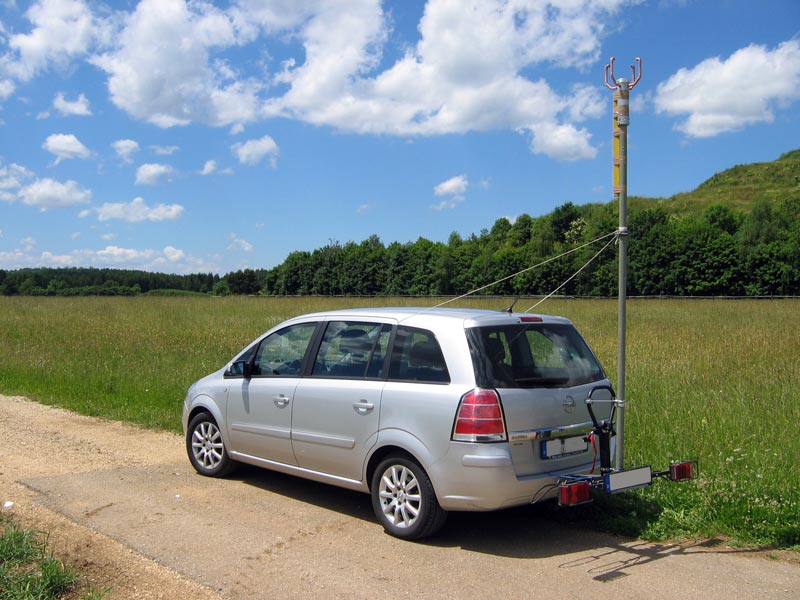
Picture: Car as a substitute wind tunnel
Finally, the use of an auxiliary wind tunnel in the form of a moving car with calm.
The fiberglass mast is 3 meters high. With the measurement are taped at the same time the speed of the car with GPS and the wind data.
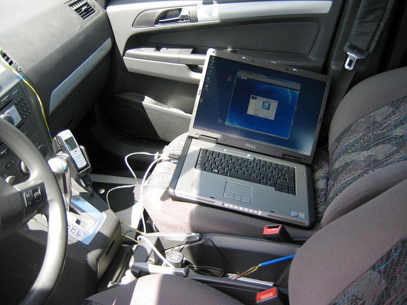
Picture: Data recording.
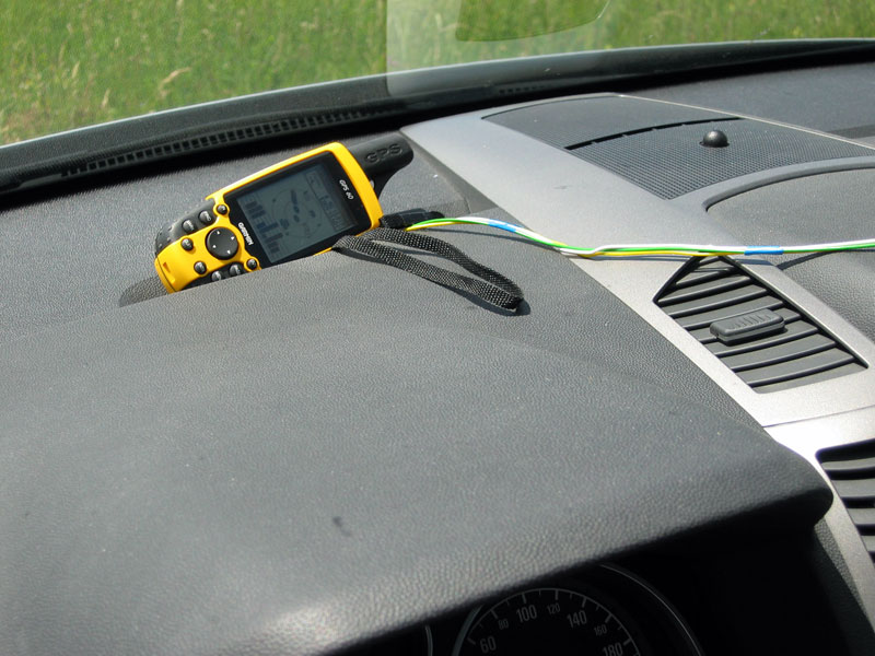
Picture: GPS in the car
The speed of the car is measured with gps. The "text out"-format is used by the Garmin GPS.
This spends among other things the speed in three space vectors apart with a resolution of 0.1 m/s every second once more.
Picture: Extract of a log file in a test journey
Meaning of the columns 1: Time (UTC), 2: Speed investigates with GPS [m/s],, 3: Speed anemometer [m/s], 4: Wind direction [°], 5: Virtually temperature anemometer [°C], 6: Number of valid measurements in 1/4 seconds (max. 25), 7: Number of internal corrections type V (debug), 8: Number of internal corrections type C (debug), 9: Number of mistakes difference in temperature X and Y, 10: Number of mistakes by too fast changing temperature,, 11: Number of distance failure X, 12: Number of distance failure Y, 13: Temperature in the Measuring arm north (for heating), 14: Filament current [mA], 15: Real-time if > 0 (debug)
By the cooperation with a famous German manufacturer of meteorological measuring instruments, I could use its professional wind tunnel.
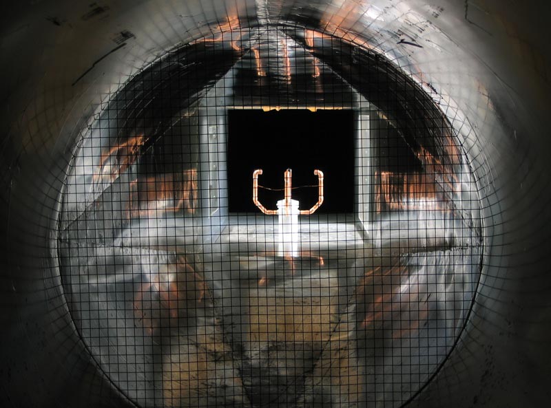
Picture: Look through the wind tunnel onto the anemometer.
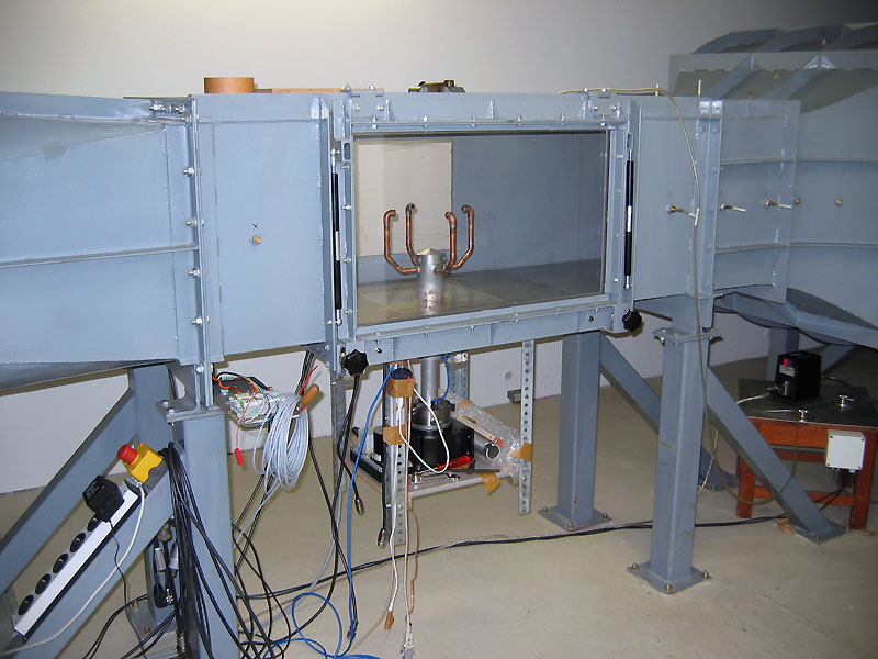
Picture: Anemometer within the wind tunnel.
Picture: Look along the wind tunnel.
The measurement and correction of the wind speed and direction dependent reductions in an ultrasonic anemometer represent a large challenge.
Just the mechanical dimensions of the selected construction appear here as unfavorable. Clear corrections are necessary.
The shown values have been measured while the calibration with the auxiliary wind tunnel in many hours. I drove over 150 km with the shown vehicle assembly!
Picture: Direction dependent correction factors a(φ) as a diagram (on top is the north).
With the values which were won in the professional wind tunnel, this correction can be further refined.
The chosen construction form is close to the type described in the literature [5] (ATI-type; Kaimal and Gaynor, 1983).
Under use in the literature [1] described properties an equation is determined:
Vm/Vt = 1 - (β * Um-γ) * (57 - φ) / φ , (0 ≤ φ ≤ 57) , β=0.61 , γ = 0.335
Vm/Vt = 1 , (57 < φ ≤ 90)
Picture: Factor Vm/Vt (Vm,φ) of the wind direction and wind speed dependent correction.
Here some literature places (unfortunately, not all free of charge and the addresses change from time to time):
The wind direction is iteratively calculated with the corrected values.
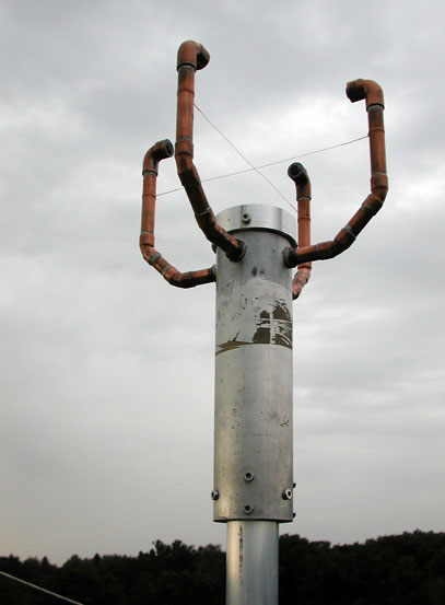
Half a year the anemometer was built on an approx. 30 m high mast.
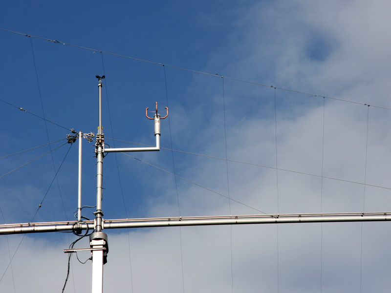
Picture: Anemometer in autumn
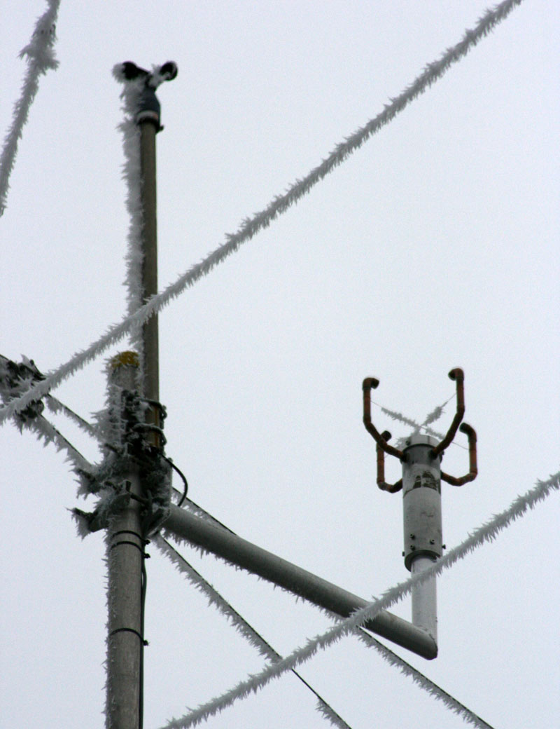
Picture: In winter the heating keeps the anemometer ice-free. Only the protection of birds is covered with ice.
Picture: Measurement of the wind speed (24 hours) with the ultrasonic anemometer (gusts 3 seconds according to WMO).
Picture: Measurement of the wind speed with a conventional wind gauge for comparison (gusts 1 second not according to WMO).
Picture: Comparison of the indicated wind directions between the ultrasonic anemometer and a conventional weather vane (the same period 24 hours).
On the graphics, one can easily recognize the inadequacy of a mechanical system in the form of the approach values. The ultrasonic anemometer works perfectly.
Final result at 12th April 2009 after more than a half year and 8,100,000,000 (eight-point-one-billion) measurements:
For comparison, there is a cup anemometer.
The correlation factor of the minute averages: 0.9998
The correlation factor of the 3-seconds gust of wind (each minute): 0.9994
Highest / the lowest virtual temperature: 28.7 °C / -11.2 °C
The project was much more difficult than imagined. But I think the result is brilliant.
The aimed exactness and all mechanical and electric qualities were reached as specified.
Now this does not mean that all desirable qualities exist completely. There are enough qualities
which do not appear in the specification!
The extreme small bandwidth of the sound converters admits no other signal processing with this electronic circuit.
This leads to an only restricted security of the detection of the envelope curve which must be
secured by a Kalman-filter.
And this leads to an essential problem at the start or by interruptions of the measurement.
Nevertheless, for the first prototype it has succeeded already very much. But there still remain enough improvement possibilities.
Several years have passed and many ultrasonic anemometers are now available, some of them quite cheap. But the charm of the special has not completely disappeared.
I have yet to find another successful design from private individuals or universities.
There was still enough to improve, and now the possibility of using my institute's wind tunnel has given me the impetus to develop an advanced prototype.
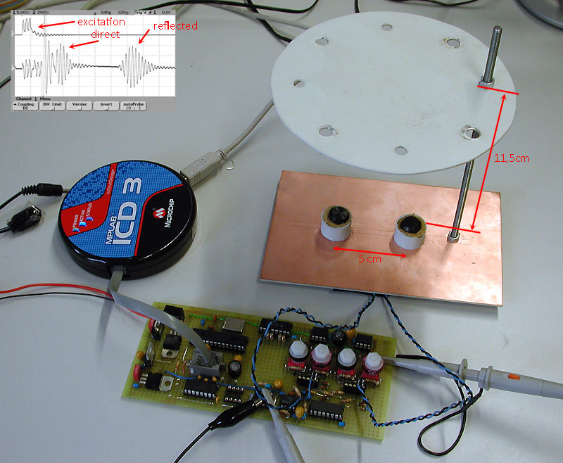
Picture: Sound propagation paths
Separation of direct and indirect sound using transducers with a wide dispersion angle.
The sound converters used (40 kHz) have a very large dispersion angle. This causes the direct and indirect sound to overlap. To separate the two, the path around the reflector must be much longer than the direct path. This results in a very high reflector and therefore a very sharp corner α of the sound propagation path. By the time the indirect sound actually used for the measurement arrives, the direct sound must have faded away completely. The sharper the corner α, the less influence the wind has on the propagation time of the sound.
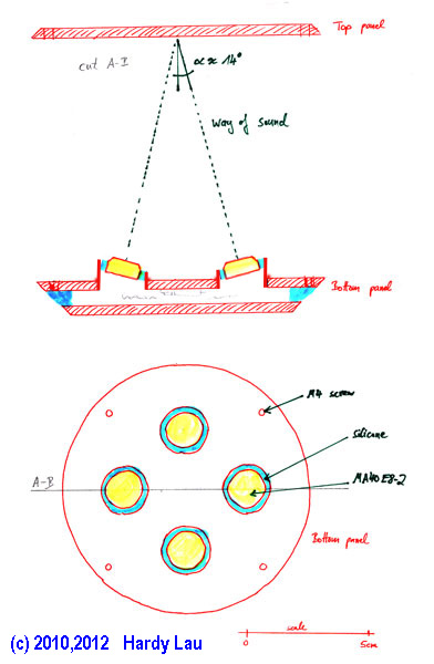 Picture: A sketch of the new mechanical design to reduce the turbulence. Only the bottom plate has to be heated in winter. |
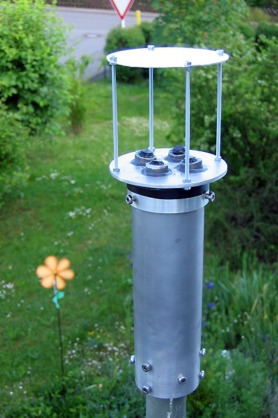 Picture: The second prototype with measurement by a reflector. |
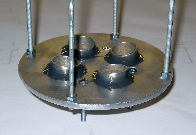
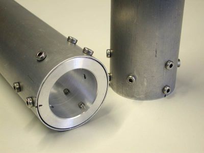
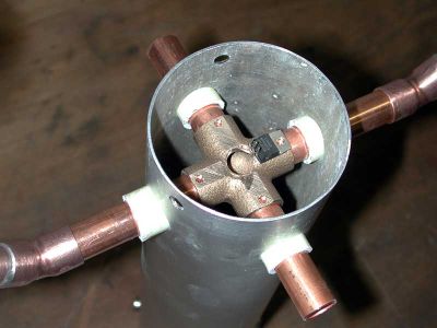
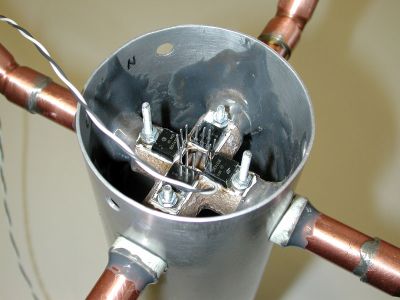
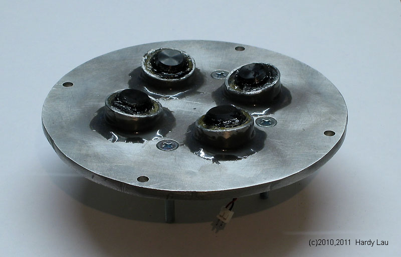
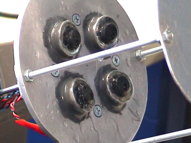
Picture: Detailed picture of the base plate
The tube sockets (aluminum) are soldered into the base plate because of better heat conductivity. Because the soldering of the aluminum has not succeeded perfectly the solder joints are sealed in addition with 3M Scotch-Weld 2216 B/A.
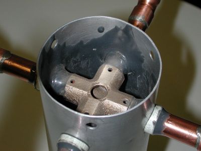
Picture: Detailed picture of the sound converter arrangement
With this new fixing of the sound converters, there are no problems at the strong rain.
The ultrasonic converters are glued slantwise (in the direction of sound propagation) with transparent and ultraviolet resistant silicone (WEICON Flex + bond)
into the tube sockets of the heatable base plate.
The ultrasonic signals are distinguished by this connection and arrangement of the ultrasonic converters.
As to itself pointed later, the observance of the installation corner is important. Otherwise, an asymmetry arises which must be compensated with an extensive calibration.
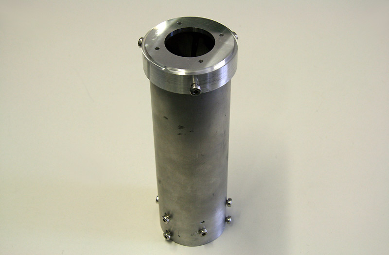
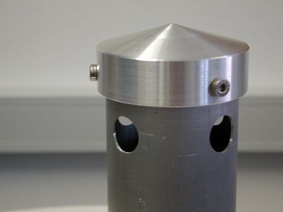
Picture: Cabinet without measuring setup.
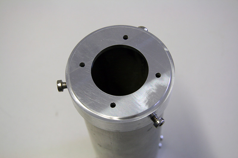
Picture: The upper disk for the connection of the measuring setup.
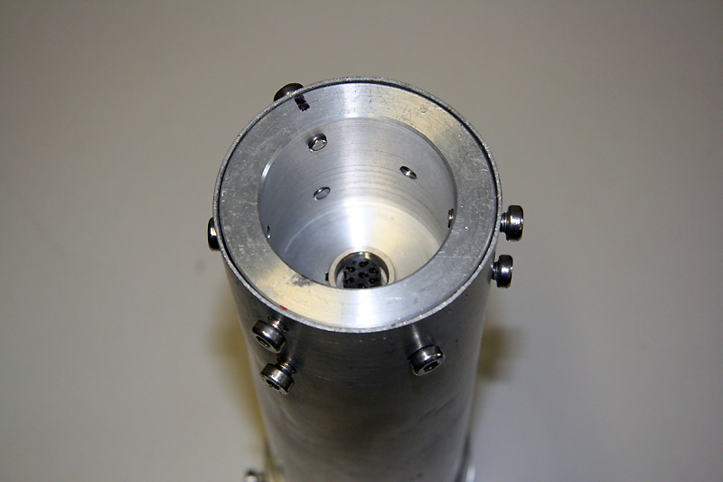
Picture: The mast's fixture with plug connection.
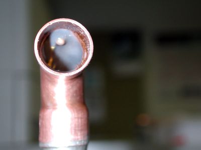
Picture: New sound propagation way indirectly about a reflector
With this new design, the sound spreads out directly and at the same time indirectly about the reflector. The sharp corner serves to distinguish time wise direct from the indirect sound. The wind to be measured favors above others or, besides, decreases only proportionately the run time of the sound signals depending on the corner α.
with distance d between the converters and the reflector, speed of sound c, angle α,
wind speed v, run time of the sound forward tforward and run time of the sound back tback.
with distance d between the converters and the reflector, speed of sound c, angle α, wind speed v,
run time of the sound forward tforward and run time of the sound back tback.
Hence, the noise is also bigger accordingly. The optimum angle would be 45 degrees if then the direct sound did not interfere. An essential advantage is that the wind is almost unhindered from the sound converters and the aerial whirls of the sending sound converter hit the receiver's sound converter not directly. The corner between the wind and the surfaces of the sound converters remains always acute.
The other calculations for the whole wind speed and direction are the same like with the first prototype. Please, read up in the upper part.
Picture: New electronics
New electronic board (with Microchip dsPIC33fj128mc802 as new processor).
Four transformers are remarkable on top on the right. Together with the driver stages, the biggest updates are towards the predecessor.
This time, the microprocessor offers 34 MAC/MIPS computer power and a 12-bit A/D-converter with 500,000 samples per second. I renounce the analogous zero passageway recognition this time. Now the A/D converter is supported by a DMA channel. There is up to the end of the measurement generally no interrupt. Also, the main storage is with 16 KB, and of it 2 KB of DMA memory, more than large enough. The yet more complicated signal production is managed again elegantly with the built-in PWM generator.
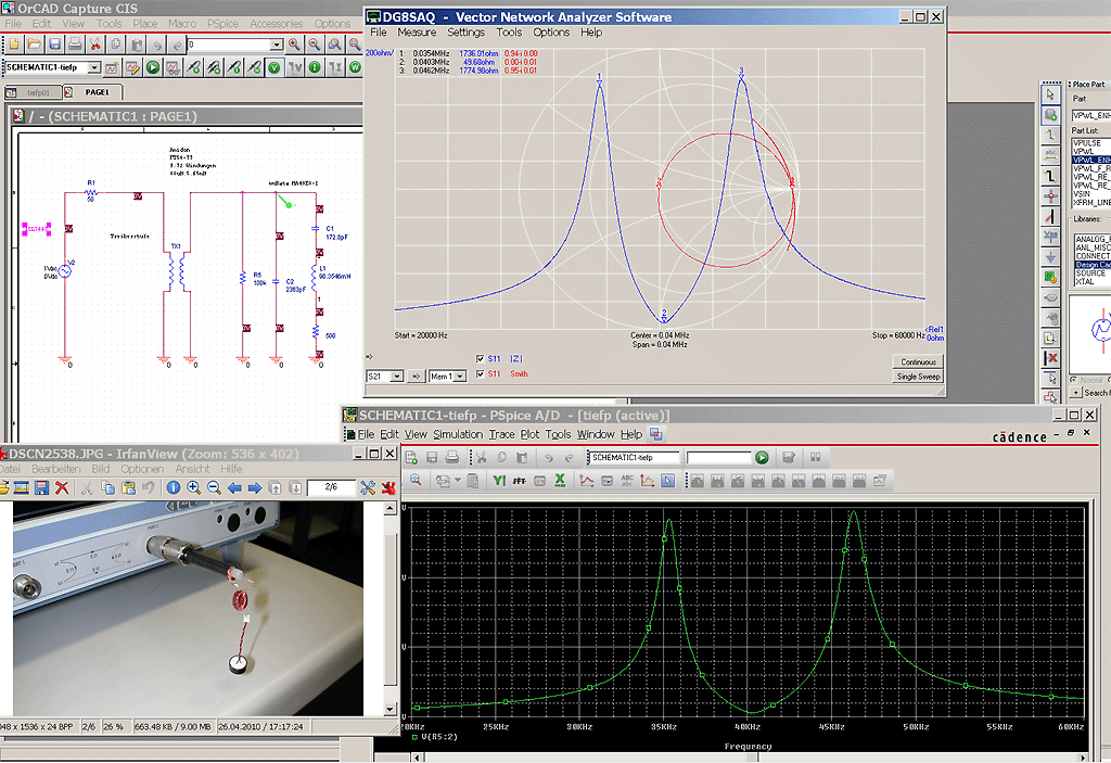
Picture: Simulation and measurement
Simulations and measurements are very close at the new development...
Quite substantially anew is the adaptation of the sound converter resulting in a larger bandwidth.
New possibilities thereby arise in the signal forming and signal processing.
Besides, the correspondence between the simulation with PSPICE and the measurement is quite amazing. Also, the simulation of the resultant receipt signals proves an extremely good correspondence to the measurement.
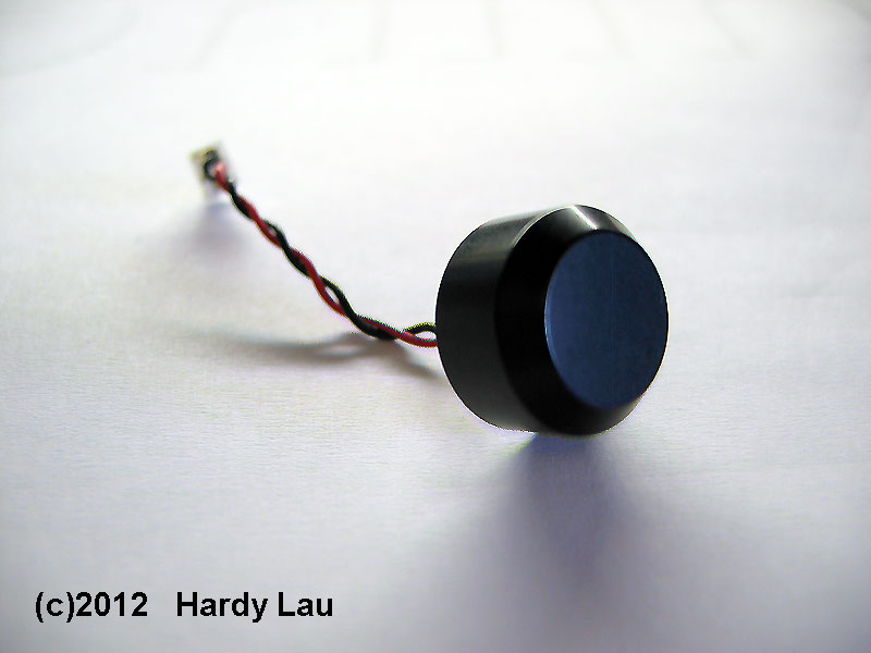
Picture: Sound transducer muRata MA40E8-2
It sounds so easy. One takes a watertight sound converter and that's it. Far from it!
In the case of closer consideration, the extreme use of this sound converter strikes with this project.
MA40E8-2 is intended for the application as a distance alert with passenger cars. There, distances must be recognized in the range 20 cm to 150 cm. Besides, the resolution or the accuracy should lie in the range ±10 cm. The wavelength of a sound wave (40 kHz) in air lies with approx. 9 mm. Hence, the quality factor of this sound converter is very high, i.e. the bandwidth very slightly. The sound beam width with approx. 90° is extra-size so a few sound converters in the bumper are sufficient.
In this application, the distance is steady here and the run time is measured. But the wind speed is measured in a resolution of 0.05 m/s (rms). This proves with ambient temperature, the sharp corner and a distance of approx. 10 cm between the sound converters and the reflector a distance of approx. 0.07 mm. A very small sound beam width would also be a strong advantage for the second prototype.
And, besides, is the accuracy which is achieved here even higher. Since this is including the influence of the turbulence in the quickly moving air. One can reach an almost unbelievable accuracy with these cheap sound converters!
And why all that?
Suitable sound converters are not available in small numbers of pieces and payable price.
Hence, the big strains with this actually very inexpedient sound converter.
Contrary to the claim on other websites, the sound transducers have a metal housing.
With the Vector-Network-Analyzer (DG8SAQ design) and the associated program, it is very easy to determine the equivalent circuit of the sound converters. This is important for the design of the driver circuit.
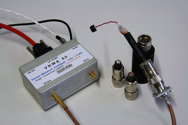
Picture: Self-assembled Vector-Network-Analyzer (DG8SAQ design).
Picture: Measurement S11 of a Murata MA40-E8-2 of the sound converter.
Picture: Equivalent circuit of the Murata MA40E8-2 of the sound converter.
The secondary inductance of the transformer forms together with the capacity of the sound converter a resonance circuit. The frequency of this resonance circuit should match the frequency of the sound converters.
Picture: Secondary inductance of the transformer
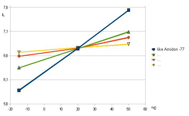
As already suggested above the temperature dependence of the secondary inductance of the transformer is a problem. A good friend examined this dependence more exactly and made this diagram. The type of the transformer which I will use now is show by the yellow curve (I have intentionally hidden the indication of the type).
The attempts have shown the interference of the signals by the changing secondary inductance clearly. However, the signal processing has functioned in the whole area of -20 °C to +60 °C nevertheless.
Picture: Part of the new schematic diagram.
The driver page was strictly separated from the receiver's page. The mute circuit could thereby be canceled. The driver stages are adapted with resonant transformers exactly to the sound converters. The analogous zero passageway detection has been canceled. Now the schematic and the simulation have occurred with OrCAD. This would also simplify a board production very much.
The correlation simplifies the signal processing considerably. It serves for the monitoring by the Mismatched filter won data. The system needs no Kalman-filter.
The construction of the coefficients of the Mismatched filter in this drought is made easier thanks to the pulse compression very much.
This filter must not evaluate anymore the wrapping shape of the signal, but the signal with pulse compression!
Picture: Correlation answer
In addition to the mismatched filter a correlation of the receipt signals (see picture) is used. With this the temperature cannot be determined, however, it is an additional security with the detection of the wind speed.
In the other charts to the correlation the abscissa always has the range to 524. This comes from 512 samples (in 1024 ms) from those the first 250 simply fallen out because there cannot appear benefits signals. With two input sequences of the correlation (the way there and way back), there originate 524 initial values. These are displayed in each case. The values of the correlation are standardized in each case, i.e. the maximum is 1.
In this version, the quick comparator has been canceled. To reach a sufficient resolution with only 500,000 samples per second, a linear interpolation is used for the determination of the zero passageways. Linear interpolation because SIN (x) ~ x for small x.
Picture: Interpolation
Besides, the resolution of the wind speed can be bigger, nevertheless, than by the speed of the A/D converter given. In addition, the average of a linear interpolation of several zero passageways of the signal is used. The number and choice of the zero passageways are made that a possible offset and, therefore, jitter, conditioned by overlapping, compensates itself. The above picture shows the samples chronologically properly, i.e. there are exactly 12.5 samples per oscillation.
A is the amplitude of sample no. 7, B is the amplitude of sample no. 8.
Then the zero passageway takes place with sample no. 7 + A / (A+B).
This became possible by the substantially bigger sampling resolution (12 bits) of the amplitudes. With the first version the amplitudes, conditioned by the low memory, had to be reduced even to 8 bits of resolution.
This version of the ultrasonic anemometer forms the average for every second. The vector average is used with speed and wind direction. The disadvantage of the unfavorable geometry with the sharp corner between wind and sound path is thereby compensated extensively.
To reduce the noise even further approx. 10% of the biggest and 10% the smallest measured data are set aside with a median filter before the average education. Smaller "outliers" are deleted with it.
Picture: Correlation answers of different suggestion signals
The correlation profits from the larger bandwidth. Different shapes of the broadcasting signal (headwords: pulse compression, barker-code) prove correlation answers with a larger distance to the side lobes. The above picture shows an essential improvement compared with the filter answer of the best Mismatched filter in the first version of the ultrasonic anemometer. I intentionally do not show the accompanying broadcasting signals.
This correlation must not evaluate anymore the wrapping shape of the signal, but the signal with pulse compression!
Even further improvements are possible with the sending signal. However, these require an advanced dynamic adaptation at the run time. Up to now up to an adaptation of the frequency to the temperature way of the sound converters I renounce this.
In a measuring cycle different pulse forms are used by now. Every pulse form has its special advantages. One has a good phase stability of the receipt signal, the above one a good suppression of the side lobes with the correlation of the receipt signals.
Picture: Correlation answer
The animation shows the normalized correlation of the receipt signals with wind speeds of -30 m/s to +30 m/s in steps of 5 m/s. The air temperature amounts to approx. 21 °C.
The distance to the side lobes is large enough at all wind speeds.
Picture: The first lab construction
The first tests with the new construction and mathematical signal processing.
Now as debugger the quicker Microchip MPLAB ICD3 is used.
With an exact look at the signal in the above picture, one can immediately ascertain the immense difference.
The sound converters are inserted now nearly level. What happens, actually, with rain?
Picture and film: Rain attempt
This video (20 mb, WMV) shows the rain attempt. In addition, the sound converters were loaded directly with a drop of water.
Picture: Measured wind speed with rain.
The influencing of a raindrop is possibly low and only from short duration. At snowfall the sound converters and the lower disk are heated, in addition.
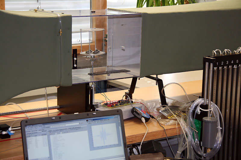
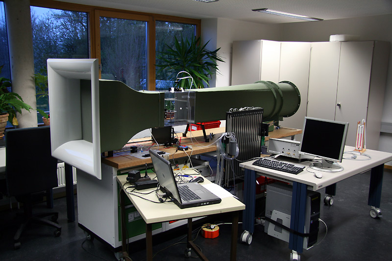
Picture: New wind tunnel
This small wind tunnel GUNT HM 170 (2.25 kW, ~28 m/s 292mm*292mm) is available since autumn 2010 for further development. Datasheet of the wind tunnel.
This new wind tunnel was the reason to develop again a new anemometer. Even if this wind tunnel is very small, development gets easier a hundred times and faster than with the possibilities during the years before. Months of working time become hours!
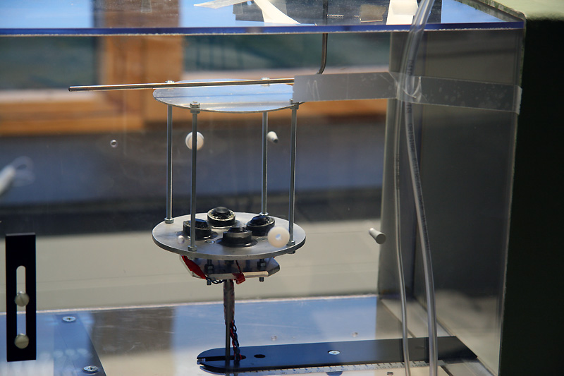
Picture: The second prototype of the anemometer with tests in the wind tunnel (Spring 2012).
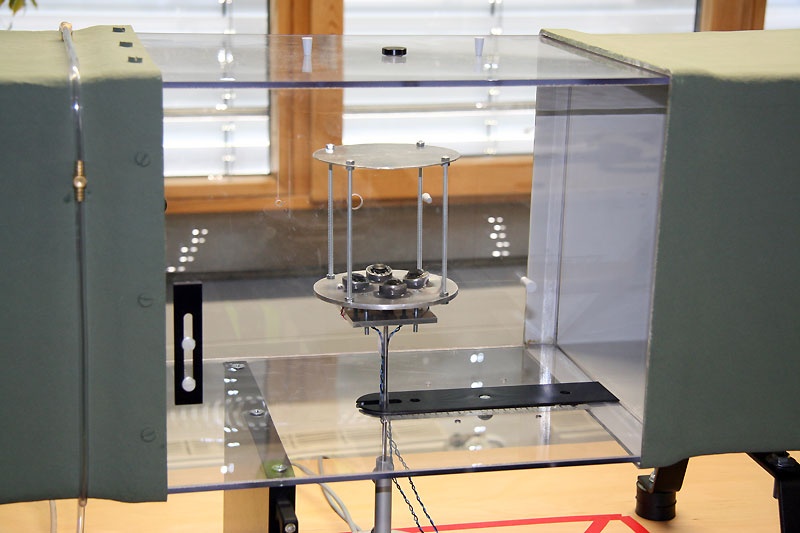
Picture: The second prototype of the anemometer with tests in the wind tunnel (Spring 2012).
Picture and film: Anemometer with a measurement in the wind tunnel
The video (10 mb, WMV) shows the anemometer with a measurement in the wind tunnel.
The auditory protection does not lie around there pointlessly!
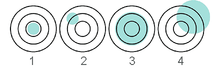
Picture: Precision, correctness and exactness
The precision is a measure of the correspondence between independent measuring results under firm conditions. Lying several measuring values close together, so the measuring method has a high precision. However, this does not mean yet that the measured values are also right.
The correctness is a measure of the correspondence between the average preserved from a big record and the approved authoritative value. If the average from many measurements well agrees to the true value, the correctness is high. This says nothing about how strongly the single values scatter.
The exactness is a measure of the correspondence between the (single) measuring result and the true value of the measuring size. One can reach a high exactness only if the precision, as well as the correctness are good.
In the above picture is with it: 1 = exactly with good correctness, 2 = exactly with bad correctness,
3 = imprecise with good correctness, 4 = imprecisely with bad correctness.
Most manufacturers give very uncertain information to the exactness of her devices. Thus, only the rms value is given as a rule.
By a Gauss distribution corresponds the standard deviation δ to the root-mean-square value (rms).
Then there are 68.3% of all measuring values in the area ± δ, 95.5% of all measuring values in the
area ±2δ and 99.7% of all measuring values in the area ±3δ.
Ultrasonic anemometers are not very exact. Hence, you should not be also used to the achievement forecast by wind strength arrangements.
With knowledge about these circumstances, you should look at the information to the exactness of this device and all other commercial devices.
Picture: During the calibration
The wind tunnel offers an area of 20 cm * 20 cm at a wind speed of more exactness than 2% up to 28 m/s.
Because the sound waves are reflected in the wind tunnel the measuring rate is reduced during the calibration a little. This does not interfere in the normal operation.
Picture: Anemometer and Pitot - static tube to the comparative measurement
A Pitot - static tube serves for the measurement of the wind speed in the wind tunnel together with an electronic difference pressure gauge, barometer, thermometer, and hygrometer.
The function, but not the exactness, up to approx. 40 m/s wind speed can be checked with an applicable cross section reduction (for the Bernoulli experiment).
Picture: The measured speed at the scheduled values (5,10,15,20,25 m/s) about the measured wind direction.
This almost quite insignificant diagram contains 360 single measurements. Even with a very short integration time, one needs approximately 1 minute per measuring point. These are 6 working hours!
With these values, a two-dimensional table is put on in the anemometer and after the measurement, the corresponding corrected value is displayed.
Unfortunately, the mechanically low precision with the construction and the small distance between the sound converters together with the sharp corner between the wind and sound way are reflected in the attainable accuracy. The specified values can be just still reached.
Picture: Measurement after the calibration.
A measuring value per second with 28.1 m/s.
The anemometer was slowly turned by hand once around the axis.
Result: Average 28.06 m/s and standard divergence 0.37 m/s (=1.3%).
Picture: Measurement after the calibration.
A measuring value per second with 5.0 m/s.
The anemometer was slowly turned by hand once around the axis.
Result: Average 4.99 m/s and standard divergence 0.3 m/s and with it just still within the specification.
Picture: Measurement after the calibration.
A measuring value per second (300 seconds) with calm.
Result: Standard divergence 0.25 m/s.
One can presumably observe a resonance effect here. The standard deviation is with wind speeds more than 2 m/s clearly lower than with absolute calm.
Picture: Measurement of the wind speed in the main axis (0°).
This main axis is the utmost exact place in the whole range. The standard deviation amounts here to 1.4%.
Picture: Divergence of the wind direction.
The standard deviation of the wind direction δα = arctan( δV / V0).
| V0 | δα |
|---|---|
| <1 m/s | No direction processed |
| 2 m/s | 2.8° |
| >5 m/s | <2.0° |
The measurement of the wind direction is influenced with this prototype something by the inexact geometry.
Picture: Measurement of the wind speed and wind direction with 15 m/s and an angle of 23.5° for a period of 300 seconds.
Picture: Distribution chart of wind speed @ 15 m/s.
The standard deviation of the wind speed amounts to 0.1 m/s.
The standard deviation of the wind direction amounts to 0.5°.
Picture: Measurement of the wind speed and wind direction with 5 m/s and an angle of 30.0° for a period of 300 seconds.
Picture: Distribution chart of wind direction @ 5 m/s.
The standard deviation of the wind speed amounts to 0.1 m/s.
The standard deviation of the wind direction amounts to abt. 0.6°.
It really concerns a normal distribution with the wind speed and with the wind direction.
With the wind, speed there are 72.2% of all measuring values within ±δ,
94.0% of all measuring values within ±2δ and 99.5% of all measuring values within ±3δ.
With the wind direction, there are 75.6% of all measuring values within ±δ,
94.0% of all measuring values within ±2δ and 99.4% of all measuring values within ±3δ.
The development of the program was much easier in spite of adaptations to the new hardware (e.g., DMA) and was quicker than before.
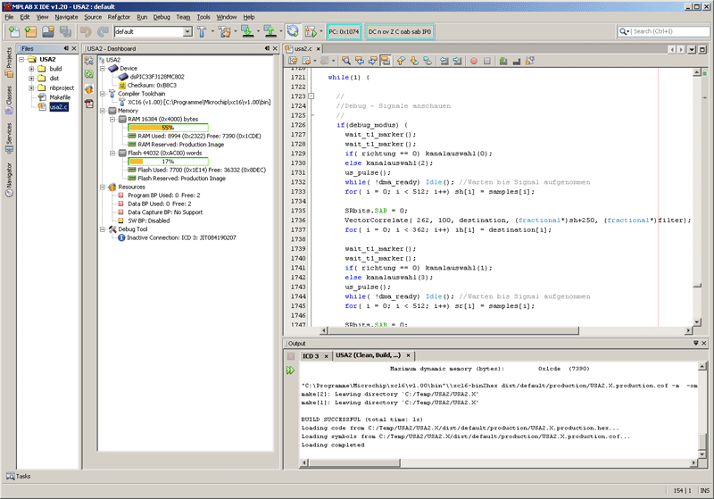
Picture: Snapshot of the development system
Now Microchip MPLAB X IDE v2.30 and MPLAB XC16 v1.24 compiler are used.
The microcontroller program is widely finished. As one can see this time still a lot of places are free in the program memory and data memory. The program written in C exists of approx. 2000 lines and intensely uses the high optimized functions of the DSP-Library.
There are still possible improvements, however, not realized in this version. Sound converters with higher frequency have a bigger absolute bandwidth and a substantially smaller angle of radiation. The direct sound and the reflected sound would not overlap anymore. A temporal separation by using a small corner between the wind and sound directions would become needlessly. Then the distance to the reflector could be clearly smaller. Unfortunately, high-frequency versions of the sound converters need an adaptation of the acoustic impedance to the air. This adaptation is achieved by a plastic layer. This plastic has very bad heat conductivity and this leads to problems in winter. In addition, these sound converters are expensive and are only hardly available in a small number of pieces. For now, I remain with the already available sound converters with 40 kHz.
I am very contented with the result. The specification is completely kept and all other qualities correspond of their one commercially salable precision measuring instrument.
The calibration process is a little more difficult. The sound converters must be fastened in the exact spatial corner. Caused by the small distance of the sound converters the mechanical exactness must also rise to achieve equally good results. However, with an available wind tunnel, this is no problem.
Now the step for the development of a device ready to go into mass production would not be big anymore. The electronics would also fit in the first prototype very well. However, unfortunately, the wind tunnel is too small for a calibration for it.
Other projects (German language)